Sketching Layer
Introduction
‘Sketching’ is the core algorithmic foundation on which libSkylark is built, and is able to deliver faster NLA kernels and ML algorithms.
Dimensionality reduction in NLA and ML is often based on building an oblivious subspace embedding (OSE). An OSE can be thought of as a data-independent random “sketching” matrix S \in R^{s\times n} whose approximate isometry properties (with respect to a norm \|\cdot\|_p) over a subspace (e.g., over the column space of a data input matrix A, and regression target vector b) imply that,
\|S(A x - b)\|\approx\|A x-b\|
which in turn allows the regression coefficients, x, to be optimized over a “sketched” dataset - namely S*A and S*b - of much smaller size without losing solution quality significantly. Sketching matrices include Gaussian random matrices, structured random matrices which admit fast matrix multiplication via FFT-like operations, hashing-based transforms, among others.
Overview of High-performance Distributed Sketching Implementation
Sketching a matrix A typically amounts to multiplying it by a random matrix S, i.e., A * S for compressing the size of its rows (row-wise sketching) or S * A for compressing the size of its columns (column-wise sketching).
In a distributed setting, this matrix-matrix multiplication primitive (sketching GEMM operation) is special in the sense that any part of matrix S can be constructed without communication. In addition, depending on the relative sizes of A, S and the sketched matrix (output), we can organize the distributed GEMM so that no part of the largest-size matrix is communicated (SUMMA approach), thus resulting in communication savings. Further optimizing, we can perform local computations over blocks of A, S, and also assume transposed views of the operands for memory and cache use efficiency.
In particular when both A and S are distributed dense matrices we represent them as Elemental matrices and support sketching over a rich set of combinations of vector and matrix-oriented data distributions: in vector distributions different processes own complete rows of columns of the matrix that are p apart (p is the number of processes) while in matrix distributions each process owns a strided view of the matrix with strides along rows and columns being equal to the dimensions of the process grid.
In our sketching GEMM, local entries of the random matrix S are computed independently by indexing into a global stream of random values provided by a counter-based Parallel random number generator (supplied by Random123 library). No entries of S are communicated since they can be locally generated instead. A can be squarish (aka “matrix”) or tall-and-thin or short-and-fat (aka “panel”). In multiplying with S, matrix-panel, panel-matrix, inner-panel-panel or outer-panel-panel products may arise. We provide separate implementations for these cases organized around the principle of communication-avoidance for the largest of the matrix terms involved in the GEMM, for each of the input/output matrix-data distribution combinations. The user can optionally set the relative sizes that differentiate between these cases. Local S entries can be incrementally realized in a distribution format that best matches the matrix indices of the local GEMM operation that follows it. Resulting S blocks typically traverse the smallest of matrix sizes in increments that can optionally be specified by the user. This has the extra benefit of minimizing the communication volume of a collective operation that generally follows this local GEMM - essentially to compensate for the stride-indexed matrix entries in the factors.
As an example we provide a pseudocode snippet (in Python syntax) that describes the rowwise sketching of a squarish input matrix A, initially distributed across the process grid in [MC, MR] format (please refer here for a comprehensive documentation of distribution formats, here appearing in brackets): S is first realized (its random entries are actually computed in the desired distribution format - in embarrassingly parallel mode) and then the local parts of A and S are multiplied together. Finally collective communications within subsets of the process grid take place to produce the resulting sketched matrix (C[MC, MR]). The corresponding C++ code (allowing also for incremental realization of S) can be found in libskylark/sketch/dense_transform_Elemental_mc_mr.hpp.
def matrix_panel(A[MC, MR], S):
    S[MR, STAR]       = realize(S)
    C_hat[MC, STAR]   = local_gemm(A[MC, MR], S[MR, STAR])
    C[MC, MR]         = reduce_scatter_within_process_rows(C_hat[MC, STAR))
    return C[MC, MR]
Quite interestingly and depending on the distribution format of the input and sketched matrices, sketching can be communication free. The following snippet illustrates this remark when both input and sketched matrices are in [VC, STAR] or [VR, STAR] distribution formats - same scenario as before, rowwise sketching of a squarish input matrix:
def matrix_panel(A[VC/VR, STAR], S):
    S[STAR, STAR]     = realize(S)
    C[VC/VR, STAR]    = local_gemm(A[VC/VR, STAR], S[STAR, STAR])
    return C[VC/VR, STAR]
Sparse matrices A are currently represented as CombBLAS matrices. As for dense sketch matrices, any part of the sparse sketch matrix can be realized without communication. Since the sketch matrix is sparse, we only require a “sparse” realization of the sketch matrix S and the sketching GEMM can be computed on the random stream directly. Similar to the SUMMA approach for dense matrices we select what will be communicated depending on input and output dimensions.
It is possible to sketch from a sparse matrix to a dense (and vice versa). The only restriction when using CombBLAS is that total number of processors has to be a square number.
libSkylark’s Sketching Layer
The purpose of the sketching layer is to provide optimized implementations of various sketching transforms and for various matrix arrangement in memory (e.g. local matrices, distributed matrices, sparse matrices ...). The majority of the sketching library is implemented in C++, but it is accessible in Python through skylark.sketch.
Sketching Transforms
The following table lists the sketching transforms currently provided by LibSkylark. These transforms are appropriate for specific downstream tasks, e.g. l2-regression, l1-regression, or kernel methods.
The implementations are provided under libskylark/sketch.
| Abbreviation | Name | Reference |
|---|---|---|
| JLT | Johnson-Lindenstrauss Transform | Johnson and Lindenstrauss, 1984 |
| FJLT | Fast Johnson-Lindenstrauss Transform | Ailon and Chazelle, 2009 |
| CT | Cauchy Transform | Sohler and Woodruff, 2011 |
| MMT | Meng-Mahoney Transform | Meng and Mahoney, 2013 |
| CWT | Clarkson-Woodruff Transform | Clarkson and Woodruff, 2013 |
| WZT | Woodruff-Zhang Transform | Woodruff and Zhang, 2013 |
| PPT | Pahm-Pagh Transform | Pahm and Pagh, 2013 |
| ESRLT | Random Laplace Transform (Exp-semigroup) | Yang et al, 2014 |
| LRFT | Laplacian Random Fourier Transform | Rahimi and Recht, 2007 |
| GRFT | Gaussian Random Fourier Transform | Rahimi and Recht, 2007 |
| FGRFT | Fast Gaussian Random Fourier Transform | Le, Sarlos and Smola, 2013 |
Sketching Layer in C++
The above sketch transforms can be instantiated for various combinations of distributed and local, sparse and dense input matrices and output sketches. The following table lists the input-output combinations currently implemented in the C++ sketching layer.
In the table below, LocalDense refers to Elemental sequential matrix type, while STAR/STAR, VR/STAR, VC/STAR, STAR/VR, STAR/VC, MC/MR refer to specializations of Elemental distributed matrices. Each specialization involves choosing a sensical pairing of distributions for the rows and columns of the matrix: * CIRC : Only give the data to a single process * STAR : Give the data to every process * MC : Distribute round-robin within each column of the 2D process grid (M atrix C olumn) * MR : Distribute round-robin within each row of the 2D process grid (M atrix R ow) * VC : Distribute round-robin within a column-major ordering of the entire 2D process grid (V ector C olumn) * VR : Distribute round-robin within a row-major ordering of the entire 2D process grid (V ector R ow)
LocalSparse refers to a libSkylark-provided class for representing local sparse matrices, while DistSparse refers to CombBLAS sparse matrices.
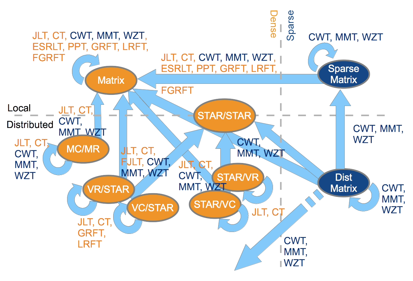 Schematic views of input and output types for various sketch transforms.
The blue color marks sparse matrix or
transforms, orange is used for dense matrix or
transforms.
Schematic views of input and output types for various sketch transforms.
The blue color marks sparse matrix or
transforms, orange is used for dense matrix or
transforms.Note
In the near future the local dense matrix will be replaced by CIRC/CIRC and STAR/STAR matrices.
Sketching Transforms
- type class skylark::sketch::sketch_transform_t<InputMatrixType, OutputMatrixType>
Query dimensions
- int get_N() const
Get input dimension.
- int get_S() const
Get output dimension.
Sketch application
- void apply(const InputMatrixType& A, OutputMatrixType& sketch_of_A, columnwise_tag dimension) const
Apply the sketch transform in column dimension.
- void apply(const InputMatrixType& A, OutputMatrixType& sketch_of_A, rowwise_tag dimension) const
Apply the sketch transform in row dimension.
Serialization
- boost::property_tree::ptree to_ptree() const
Serialize the sketch transform to a ptree structure.
- static sketch_transform_t* from_ptree(const boost::property_tree::ptree& pt)
Load a sketch transform from a ptree structure.
Accessors
- const sketch_transform_data_t* get_data()
Get the underlaying transform data.
The sketch transformation class is coupled to a data class that is responsible to initialize and provide a lazy view on the random data required when applying the sketch transform.
The sketching direction is specified using the following types:
Using the C++ Sketching layer
To get a flavour of using the sketching layer, we provide a C++ code snippet here where an Elemental 1D-distributed matrix is sketched to reduce the column dimensionality (number of rows). The sketched matrix – the output of the sketching operation – is a local matrix. The sketching is done using Johnson-Lindenstrauss (JLT) transform.
#include <elemental.hpp>
#include <skylark.hpp>
...

/* Local Matrix Type */
typedef El::Matrix<double> MatrixType;

/* Row distributed Matrix Type */
typedef El::DistMatrix<double, El::VC, El::STAR> DistMatrixType;

 /* Initialize libSkylark context with a seed */
skylark::base::context_t context (12345);

/* Row distributed Elemental Matrix A of size N x M */
El::DistMatrix<double, El::VR, El::STAR> A(grid);
El::Uniform (A, N, M);

/* Create the Johnson-Lindenstrauss Sketch object to map R^N to R^S*/
skys::JLT_t<DistMatrixType, MatrixType> JLT (N,S, context);

/* Create space for the sketched matrix with number of rows compressed to S */
MatrixType sketch_A(S, M);

/* Apply the sketch. We call this columnwise sketching since the column dimensionality is reduced. */
JLT.apply (A, sketch_A, skys::columnwise_tag());
Python Sketching Interface
Skylark also provides pure Python implementations of the various transforms, which it will default in case the C++ layers of Skylark are not compiled. Some transforms are currently implemented only in Python, but there are plans to implement them in C++ as well. Likewise, some transforms currently implemented in the C++ layer will be extended to Python in near-term releases.
Skylark uses external libraries to represent distributed matrices. For dense distributed matrices it uses Elemental. Currently it uses the c-types interface of Elemental, so be sure install that as well. For sparse distributed matrices it uses CombBLAS interfaced through KDT.
The lower layers use MPI so it is advisable an MPI interface to Python be installed. One option is to use mpi4py.
The following table lists currently supported sketching transforms available through Python.
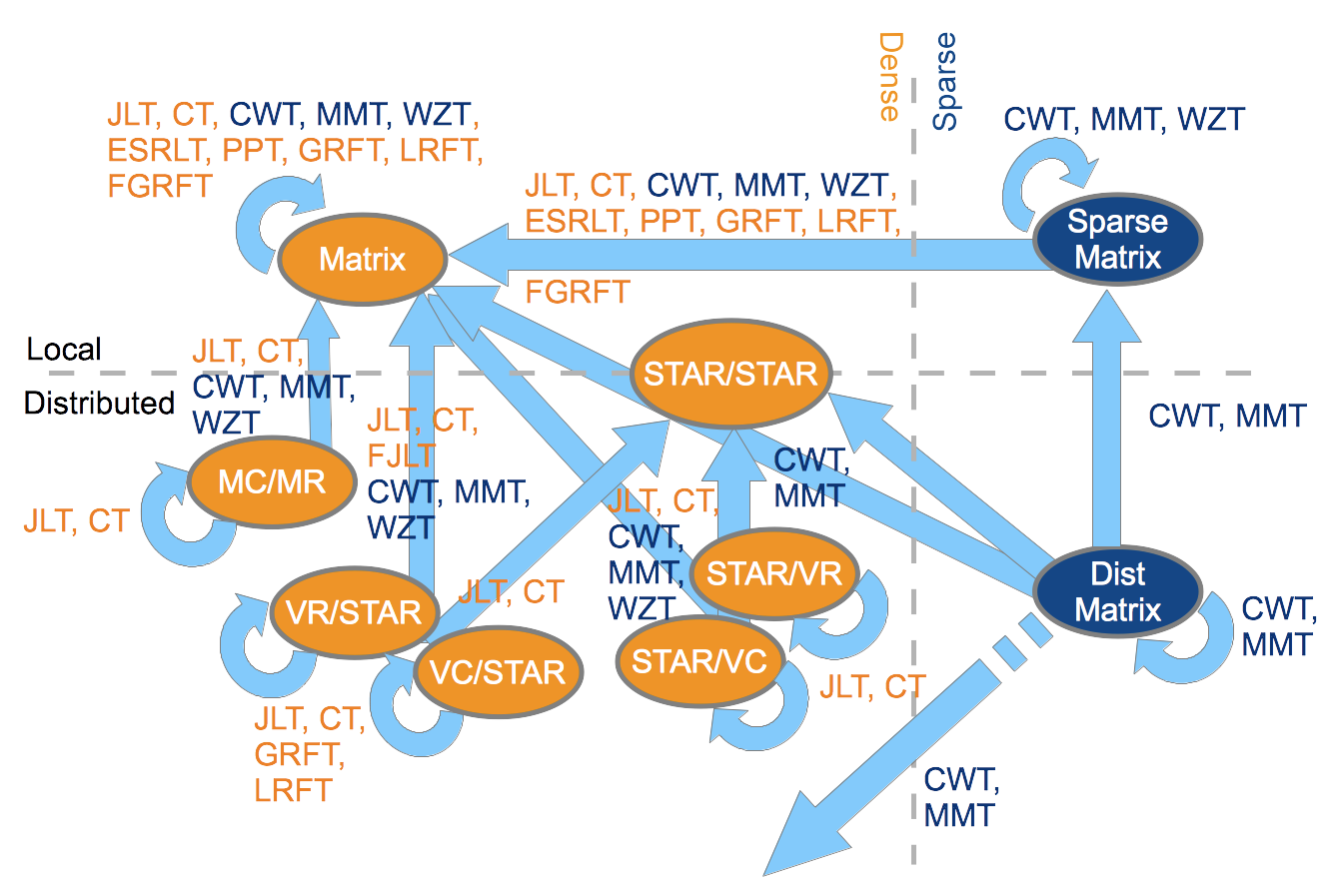 Schematic views of input and output types for various sketch transforms.
The blue color marks sparse matrix or
transforms, orange is used for dense matrix or
transforms.
Schematic views of input and output types for various sketch transforms.
The blue color marks sparse matrix or
transforms, orange is used for dense matrix or
transforms.Note
In the near future the local dense matrix will be replaced by CIRC/CIRC and STAR/STAR matrices.
Using the Python interface
Skylark is automatically initialized with a random seed when you import sketch. However, you can reinitialize it to a specific seed by calling initialize. While not required, you can finalize the library using finalize. However, note that that will not cause allocated objects (e.g. sketch transforms) to be freed. They are freed by the garbage collector when detected as garbage (no references).
Python sketch classes inherit from the SketchTransform class.
Specific python sketch classes are documented below.
Python Examples
Sketching Dense Distributed Matrices
#!/usr/bin/env python
# MPI usage:
# mpiexec -np 2 python skylark/examples/example_sketch.py

# prevent mpi4py from calling MPI_Finalize()
import mpi4py.rc
mpi4py.rc.finalize   = False

import El
from skylark import sketch, elemhelper
from mpi4py import MPI
import numpy as np
import time

# Configuration
m = 20000;
n = 300;
t = 1000;
#sketches = { "JLT" : sketch.JLT, "FJLT" : sketch.FJLT, "CWT" : sketch.CWT }
sketches = { "JLT" : sketch.JLT, "CWT" : sketch.CWT }

# Set up the random regression problem.
A = El.DistMatrix((El.dTag, El.VR, El.STAR))
El.Uniform(A, m, n)
b = El.DistMatrix((El.dTag, El.VR, El.STAR))
El.Uniform(b, m, 1)

# Solve using Elemental
# Elemental currently does not support LS on VR,STAR.
# So we copy.
A1 = El.DistMatrix()
El.Copy(A, A1)
b1 = El.DistMatrix()
El.Copy(b, b1)
x = El.DistMatrix(El.dTag, El.MC, El.MR)
El.Uniform(x, n, 1)
t0 = time.time()
El.LeastSquares(A1, b1, El.NORMAL, x)
telp = time.time() - t0

# Compute residual
r = El.DistMatrix()
El.Copy(b, r)
El.Gemv(El.NORMAL, -1.0, A1, x, 1.0, r)
res = El.Norm(r)
if (MPI.COMM_WORLD.Get_rank() == 0):
  print "Exact solution residual %(res).3f\t\t\ttook %(elp).2e sec" % \
      { "res" : res, "elp": telp }

# Lower-layers are automatically initilalized when you import Skylark,
# It will use system time to generate the seed. However, we can
# reinitialize for so to fix the seed.
sketch.initialize(123834);

#
# Solve the problem using sketching
#
for sname in sketches:
  stype = sketches[sname]

  t0 = time.time()

  # Create transform.
  S = stype(m, t, defouttype="SharedMatrix")

  # Sketch both A and b using the same sketch
  SA = S * A
  Sb = S * b

  # SA and Sb reside on rank zero, so solving the equation is
  # done there.
  if (MPI.COMM_WORLD.Get_rank() == 0):
    # Solve using NumPy
    [x, res, rank, s] = np.linalg.lstsq(SA.Matrix().ToNumPy(), Sb.Matrix().ToNumPy())
  else:
    x = None

  telp = time.time() - t0

  # Distribute the solution so to compute residual in a distributed fashion
  x = MPI.COMM_WORLD.bcast(x, root=0)

  # Convert x to a distributed matrix.
  # Here we give the type explictly, but the value used is the default.
  x = elemhelper.local2distributed(x, type=El.DistMatrix)

  # Compute residual
  r = El.DistMatrix()
  El.Copy(b, r)
  El.Gemv(El.NORMAL, -1.0, A1, x, 1.0, r)
  res = El.Norm(r)
  if (MPI.COMM_WORLD.Get_rank() == 0):
    print "%(name)s:\tSketched solution residual %(val).3f\ttook %(elp).2e sec" %\
        {"name" : sname, "val" : res, "elp" : telp}

  # As with all Python object they will be automatically garbage
  # collected, and the associated memory will be freed.
  # You can also explicitly free them.
  del S     # S = 0 will also free memory.

# Really no need to "close" the lower layers -- it will do it automatically.
# However, if you really want to you can do it.
sketch.finalize()
Sketching Sparse Distributed Matrices
#!/usr/bin/env python
# MPI usage:
# mpiexec -np 2 python skylark/examples/example_sparse_sketch.py

# prevent mpi4py from calling MPI_Finalize()
import mpi4py.rc
mpi4py.rc.finalize   = False

from mpi4py import MPI
from skylark import sketch

import kdt
import math

comm = MPI.COMM_WORLD
rank = comm.Get_rank()

# Lower layers are automatically initilalized when you import Skylark,
# It will use system time to generate the seed. However, we can
# reinitialize for so to fix the seed.
sketch.initialize(123834);

# creating an example matrix
# It seems that pySpParMat can only be created from dense vectors
rows = kdt.Vec(60, sparse=False)
cols = kdt.Vec(60, sparse=False)
vals = kdt.Vec(60, sparse=False)
for i in range(0, 60):
  rows[i] = math.floor(i / 6)
for i in range(0, 60):
  cols[i] = i % 6
for i in range(0, 60):
  vals[i] = i

ACB = kdt.Mat(rows, cols, vals, 6, 10)
print ACB

nullVec = kdt.Vec(0, sparse=False)
SACB    = kdt.Mat(nullVec, nullVec, nullVec, 6, 6)
S       = sketch.CWT(10, 6)
S.apply(ACB, SACB, "columnwise")

if (rank == 0):
  print("Sketched A (CWT sparse, columnwise)")
print SACB

# No need to free S -- it will be automatically garbage collected
# and the memory for the sketch reclaimed.

SACB = kdt.Mat(nullVec, nullVec, nullVec, 3, 10)
S    = sketch.CWT(6, 3)
S.apply(ACB, SACB, "rowwise")

if (rank == 0):
  print("Sketched A (CWT sparse, rowwise)")
print SACB

# Really no need to "close" the lower layers -- it will do it automatically.
# However, if you really want to you can do it.
sketch.finalize()